Freshwater farm planning and risk identification

What is biophysical risk?

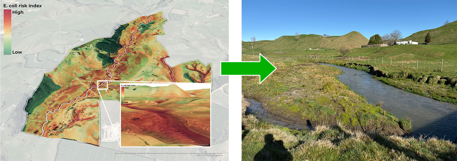
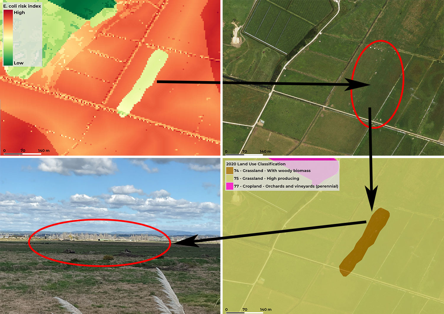
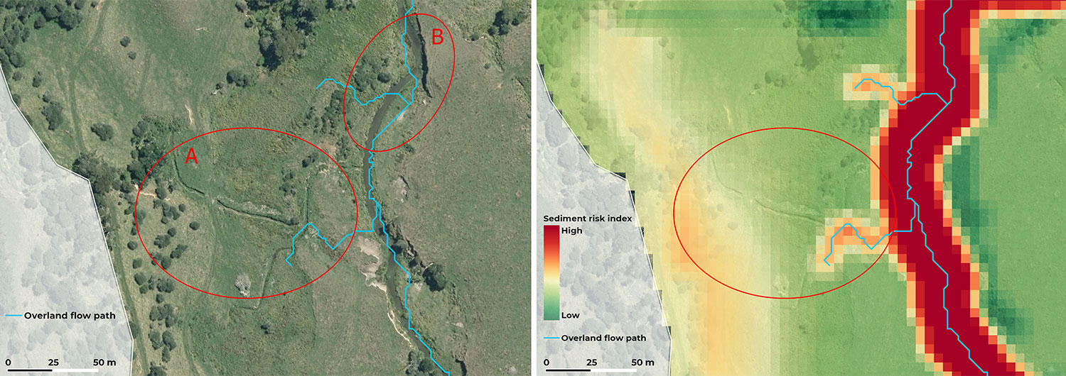
Biophysical risk (also known as inherent vulnerability) is defined as the natural characteristics of the land that contribute to contaminant loss to waterbodies. It is the attributes of the land that either can’t be changed, or can’t easily be changed, such as:

• Soil type
• Topography
• Climate
• Proximity to a stream
• Land cover.

It’s useful to remind users what biophysical risk mapping IS and what it IS NOT, to ensure that the outputs are used for their intended purpose.

Farm specific risk = inherent biophysical risk + management risk.
Understanding initial risk is important for landowners to prioritise mitigation options.

Mapping biophysical risk allows an independent, unbiased assessment of the inherent risk associated with the land. Landowners can then consider how current farm management practices interact with the inherent biophysical risks and implement best management practices or mitigations that reduce the likelihood of contaminants leaving high-risk areas and ending up in waterways.

For example, in the E. coli risk map below, red areas around the stream show a high risk for E. coli. The landowner has minimised the risk by fencing off the waterway and initiating riparian planting.

The biophysical risk maps identify risk on a 1- 5 scale (with 1 being low and 5 being high). They do not estimate nutrient loss load or water quality measurements. These measures are influenced by farm management as well as biophysical risk.

The biophysical maps are designed to help land managers or landowners interpret risk. They are only as good as the quality of the data feeding into the models. When using the maps, it is important to understand which data layers have been used to represent contaminant loss processes and their limitations. Some common limitations are
described in the following section.

Land use, and therefore land cover, is represented by LUCAS 2020 layer in the E. coli and nitrogen biophysical maps. Any recent land use changes, such as deforestation, removal of willows or conversion of pastoral land to kiwifruit, will not be represented in the biophysical maps until the underlying data is refreshed. Therefore, for some areas, the risk maps may not fully identify, or may require further interpretation to understand the true risk to waterways.

For example, in the images below, the E. coli map is identifying an area of lower risk amongst an area of high risk. However, the satellite imagery is showing a uniform pastoral area. When looking at the LUCAS layer it is picking up a grassland with woody biomass (which has a lower risk of E. coli loss to waterways). When visiting the site, you can seethat there are piles of wood debris showing recent clearing of willows.

The 2020 Land Use Map (LUCAS 2020) has a nominal mapping date
of 31 December 2020; however, mapping is based on satellite imagery captured over a range of dates over the 2020/21 summer period.

The waterways network with stream order has not been mapped in the Bay of Plenty region, therefore, a computer-generated layer was created using a process called overland flow path (OLFP). While quite good in steeper terrain, the OLFP does not always match actual waterways, like in the image below where the artificial drains are not represented (circle A), and the river takes a slightly different course to the OLFP model (circle B).

As this layer is used in the E. coli, sediment and phosphorus risk maps, what you see on the ground may not be what is represented in the biophysical risk map. The resulting sediment risk map is shown in the image below. When interpreting the risk maps, it is important to remember that if waterways are present (e.g. drains or streams), these should be treated as high-risk areas if the risk map uses proximity to waterways (or OLFP) as an input. In practice, the moderate risk area (yellow) circle C should be extended to include the artificial drains and surrounding topography.